Understanding the shape of your model is sometimes non-trivial when it comes to machine learning. Look at convolutional neural nets with the number of filters, padding, kernel sizes etc and it’s quickly evident why understanding what shapes your inputs and outputs are will keep you sane and reduce the time spent digging into strange errors. TensorFlow’s RNN API exposed me to similar frustrations and misunderstandings about what I was expected to give it and what I was getting in return. Extracting these operations out helped me get a simple view of the RNN API and hopefully reduce some headaches in the future. In this post, I’ll outline my findings with a few examples and. Firstly the input data shape: batch size is part of running any graph and you’ll get used to seeing None or ? as the first dimension of your shapes. RNN data expects each sample to have two dimensions of it’s own. This is different to understanding that images have two dimensions, RNN data expects a sequence of samples, each of which has a number of features. Lets make this clearer with an example:
import numpy as np
# Batch size = 2, sequence length = 3, number features = 1, shape=(2, 3, 1)
values231 = np.array([
    [[1], [2], [3]],
    [[2], [3], [4]]
])

# Batch size = 3, sequence length = 5, number features = 2, shape=(3, 5, 2)
values352 = np.array([
    [[1, 4], [2, 5], [3, 6], [4, 7], [5, 8]],
    [[2, 5], [3, 6], [4, 7], [5, 8], [6, 9]],
    [[3, 6], [4, 7], [5, 8], [6, 9], [7, 10]]
])
If you understand that an RNN will feed each timestep into the cell, taking the second example, the first timestep takes [1, 4] as input, second step [2, 5] etc. Understanding that even a sequence of single numbers needs to have the shape of (batch_size, seq_length, num_features) took me a while to get. If you have such a sample as a sequence of single numbers (say [[1, 2, 3], [2, 3, 4]]), you can do np.reshape(2, 3, 1) to reshape from (2, 3) into a sequence dataset
tf.nn.dynamic_rnn
To understand the output of an RNN cell, you have to think about the output of the RNN cell over the input sequence. This is where the unrolling comes from and in TensorFlow for dynamic_rnn is implemented using a while loop. If we use our data from values231 above, lets understand the output from an LSTM through a TensorFlow RNN:
import tensorflow as tf
tf.reset_default_graph()

tf_values231 = tf.constant(values231, dtype=tf.float32)
lstm_cell = tf.contrib.rnn.LSTMCell(num_units=100)
outputs, state = tf.nn.dynamic_rnn(cell=lstm_cell, dtype=tf.float32, inputs=tf_values231)

print(outputs)
# tf.Tensor 'rnn_3/transpose:0' shape=(2, 3, 100) dtype=float32
print(state.c)
# tf.Tensor 'rnn_3/while/Exit_2:0' shape=(2, 100) dtype=float32
print(state.h)
# tf.Tensor 'rnn_3/while/Exit_3:0' shape=(2, 100) dtype=float32

with tf.Session() as sess:
    sess.run(tf.global_variables_initializer())
    output_run, state_run = sess.run([outputs, state])
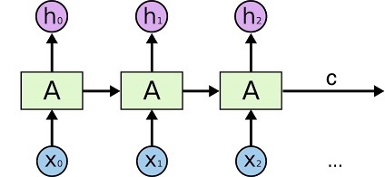
outputs: shape = (batch_size, sequence_length, numunits). If you’ve ever seen an LSTM model, this is h(t) output for every timestep (In the image below, a vector of [n0, h1, h2]. The last time step is the same value as state.h validated by running output_run[:,-1] == state_run.h. _state c and h: shape= (batch_size, num_units). This is the final state of the cell at the end of the sequence and in the image below is h2 and c

Unrolled LSTM with output [h0, h1, h2] and state output (h=h2, c=c)
This is even easier if you are using a GRUCell as state is just a single vector instead of the tuple from the LSTMCell. In this case running np.all(output_run[:,-1] == state_run) to verify the state is equal to the output at the last timestep
tf.nn.bidirectional_dynamic_rnn
The bidirectional RNN is very similar apart from obviously there is an RNN pass going both forwards and backwards through the sequence. Thus you need a cell for each separate pass and the outputs and state have a tuple pair for each RNN. In the example below, I’ve used a different num_units for the LSTM cell in each direction so it’s clear where that value is showing up in the output shape. I have also deconstructed the returned output and state into the forward and backward pairs to be clear. You may not wish to do this if you want to cleanly apply a concat operation which I will show later.
import tensorflow as tf
tf.reset_default_graph()

tf_values231 = tf.constant(values231, dtype=tf.float32)

lstm_cell_fw = tf.contrib.rnn.LSTMCell(100)
lstm_cell_bw = tf.contrib.rnn.LSTMCell(105) # change to 105 just so can see the effect in output

(output_fw, output_bw), (output_state_fw, output_state_bw) = tf.nn.bidirectional_dynamic_rnn(
    cell_fw=lstm_cell_fw,
    cell_bw=lstm_cell_bw,
    inputs=tf_values231,
    dtype=tf.float32)

print(output_fw)
# tf.Tensor 'bidirectional_rnn/fw/fw/transpose:0' shape=(2, 3, 100) dtype=float32
print(output_bw)
# tf.Tensor 'ReverseV2:0' shape=(2, 3, 105) dtype=float32
print(output_state_fw.c)
# tf.Tensor 'bidirectional_rnn/fw/fw/while/Exit_2:0' shape=(2, 100) dtype=float32
print(output_state_fw.h)
# tf.Tensor 'bidirectional_rnn/fw/fw/while/Exit_3:0' shape=(2, 100) dtype=float32
print(output_state_bw.c)
# tf.Tensor 'bidirectional_rnn/bw/bw/while/Exit_2:0' shape=(2, 105) dtype=float32
print(output_state_bw.h)
# tf.Tensor 'bidirectional_rnn/bw/bw/while/Exit_3:0' shape=(2, 105) dtype=float32

with tf.Session() as sess:
    sess.run(tf.global_variables_initializer())
    output_run, state_run = sess.run([output_fw, output_bw, output_state_fw, output_state_bw])
Understanding the outputs from the single direction RNN above, these values should make sense when thinking it’s just two RNNs. As mentioned, you may want to use the combined output state of both RNNs and concatenate the outputs. In this case, you want concat along axis=2 being the cell outputs such as tf.concat((output_fw, output_bw), axis=2, name='bidirectional_concat_outputs')
Conclusion
Without digging into applied samples and complex NLP or other sequence problems, these simple examples helped me understand the shapes of tensors passing through an RNN. And also what the output and state represent for each of these runs. I can definitely recommend taking a step back and running these operations on their own (outside of a more complex model) to more simply understand what’s going on
You can see the Jupyter notebook for my investigation at my GitHub Gist Understanding TF RNNs.ipynb